Instructions for Using Rubi
Loading the Mathematica implementation of Rubi defines an extensive system of rules capable of integrating large classes of mathematical expressions. Although Rubi’s Int commands are similar in form and function to Mathematica’s Integrate commands, the rules Rubi uses to integrate expressions do not in any way depend on Mathematica’s built-in integrator.
Loading Rubi
After the Rubi package has been properly installed as described in the Rubi installation instructions, use the command
Get["Rubi`"]
or the shorter form
<<Rubi`
to load Rubi into Mathematica.
The first time Rubi is loaded, it will take a minute or two to read in and initialize the system. However, this initial load also saves a fast loading memory image of Rubi, so all subsequent load commands will be almost instantaneous.
Options for reducing the amount of memory Rubi requires are described at the end of this page.
Integrating expressions
A Rubi command of the form Int[expn,var] integrates expn with respect to var, and returns its antiderivative (also called its indefinite integral). For example, the command
Int[x Sin[x]^2, x]
returns the antiderivative
\[\frac{x^2}{4}+\frac{\sin ^2(x)}{4}-\frac{1}{2} x \sin (x) \cos (x)\]A Rubi command of the form Int[{expn1,expn2,...},var] integrates expn1, expn2, … each with respect to var, and returns a list of their antiderivatives. For example, the command
Int[Table[x^n, {n, 0, 5}], x]
returns the list
\[\left\{x,\frac{x^2}{2},\frac{x^3}{3},\frac{x^4}{4},\frac{x^5}{5},\frac{x^6}{6}\right\}\]A Rubi command of the form Int[expn,{var,a,b}] integrates expn with respect to var, and returns the limit of its antiderivative as var approaches b minus the limit as var approaches a. According to the Fundamental Theorem of Calculus (FTOC), this difference will equal the definite integral of expn from a to b if and only if the antiderivative is continuous between the two points. For that reason, Rubi strives to return antiderivatives that are continuous on the real line to the maximum extent possible.
For example, the command
Int[x Sin[x]^2, {x, 0, Pi}]
returns $\frac{\pi ^2}{4}$ which equals the definite integral of $x \sin ^2(x)$ from 0 to pi, since the antiderivative is continuous over this interval. However, the command
Int[1/(1-x^2), {x, 0, 2}]
returns arctanh(2) although $\frac{1}{1-x^2}$ does not converge over the interval {0,2}.
Displaying integration steps
A Rubi command of the form Steps[Int[expn,var]] displays all the steps used to integrate expn with respect to var, and returns its antiderivative. For example, the command
Steps[Int[(a + b*Sqrt[x])^d, x]]
displays the steps
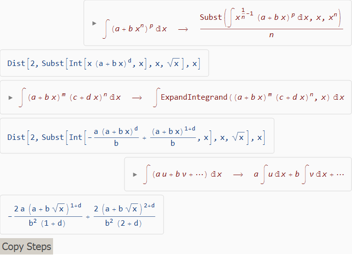
and returns the antiderivative
\[\frac{2 \left(a+b \sqrt{x}\right)^{d+2}}{b^2 (d+2)}-\frac{2 a \left(a+b \sqrt{x}\right)^{d+1}}{b^2 (d+1)}\]The boxes on the right are the integration formulas in red. The boxes on the left are the intermediate results in blue.
Click on the triangle left of a formula to display the complete integration rule including its number and application conditions. For example, clicking on the triangle left of the first formula above changes the display of integration steps to
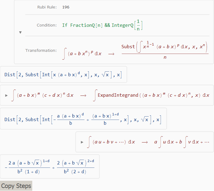
Click on an intermediate result to copy it to the clipboard so it can be entered as Mathematica input. The “Copy Steps” button copies the complete list of steps as raw Mathematica expressions as they were collected by Rubi.
A Rubi command of the form Step[Int[expn,var]] displays just the first step of the integration of expn with respect to var, and returns the intermediate result. Its display of the integration rule is the same as that used by the Steps command.
Displaying integration statistics
A Rubi command of the form Stats[Int[expn,var]] integrates expn with respect to var, and displays statistics about the integration before returning its antiderivative. For example, the command
Stats[Int[(a + b*Sqrt[x])^d, x]]
displays
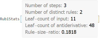
and returns the antiderivative
\[\frac{2 \left(a+b \sqrt{x}\right)^{d+2}}{b^2 (d+2)}-\frac{2 a \left(a+b \sqrt{x}\right)^{d+1}}{b^2 (d+1)}\]The Rule-size-ratio statistic is a normalized measure of the difficulty integrating an expression. It equals the number of distinct rules required to integrate the expression divided its leaf count size.
By default, Stats (as well as Steps and Step) prints its information but you can also return it for later inspection. Each entry in the Stats can then be accessed easily by either viewing the InputForm of the Stats output, or using accessor like this
{stats, result} = Stats[Int[(a + b*Sqrt[x])^d, x], RubiPrintInformation -> False];
stats["Steps"]
stats["NumberOfRules"]
stats["InputLeafCount"]
stats["OutputLeafCount"]
stats["Ratio"]
stats["Rules"]
The statistics provide the following information
"Steps": the number of steps used to integrate the expression."NumberOfRules”: the number of distinct rules used."InputLeafCount": the leaf count size of the input expression."OutputLeafCount": the leaf count size of the found antiderivative."Ratio": the rule-to-size ratio of the integration, i.e. the quotient of"NumberOfRules"and"InputLeafCount"."Rules": the rule-numbers of the distinct rules used.
To inspect integration steps or the statistics as a normal Mathematica expression instead of displaying them in a visually pleasing form, the Steps, Step, and Stats functions take an option RubiPrintInformation that can be set to False. The information about the integration is then returned together with the antiderivative. For example,
Steps[Int[x, x], RubiPrintInformation -> False]
returns
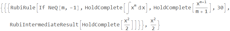
The last integer in RubiRule is the index of the integration rule applied in the list of Int’s downvalues. For example, the DownValue command
DownValues[Int][[30]]
returns the rule Rubi uses to integrate the previous example.
Global control variables
To provide options for reducing the amount of memory Rubi requires, there are two global variables that control what parts of the system are to be loaded. Therefore, to have the desired effect these control variables need to be set before Rubi is loaded into Mathematica. Their default value is True so all Rubi capabilities will be available. However:
-
If $LoadElementaryFunctionRules is False at load-time, the rules for integrating expressions involving elementary functions (e.g. log, sine, arctangent, etc.) and higher-level functions (e.g. erf, polylogarithm, etc.) are not loaded. However, the rules for integrating rational and algebraic functions are always loaded.
-
If $LoadShowSteps is False at load-time, Rubi’s ability to show the steps used to integrate expressions will not be available.